This is a listing of projects/companies working in Artificial General Intelligence (AGI). This list will grow as I come across additional projects.

  • ACT-R, led by John Anderson of Carnegie Mellon University
  • AERA, led by Kristinn Thórisson of Reykjavik University
  • AIDEUS, led by Alexey Potapov of ITMO University and Sergey Rodionov of Aix Marseille Université
  • AIXI, led by Marcus Hutter of Australian National University
  • Alice in Wonderland, led by Claes Stannegård of Chalmers University of Technology
  • Animats, a small project recently initiated by researchers in Sweden, Switzerland, and the US
  • Baidu Research, an AI research group within Baidu
  • Becca, an open-source project led by Brandon Rohrer
  • Blue Brain, led by Henry Markram of École Polytechnique Fédérale de Lausanne
  • China Brain Project, led by Mu-Ming Poo of the Chinese Academy of Sciences
  • CLARION, led by Ron Sun of Rensselaer Polytechnic Institute
  • CogPrime, an open source project led by Ben Goertzel based in the US and with dedicated labs in Hong Kong and Addis Ababa
  • CommAI, a project of Facebook AI Research based in New York City and with offices in Menlo Park, California and Paris
  • Cyc, a project of Cycorp of Austin, Texas, began by Doug Lenat in 1984
  • DeepMind, a London-based AI company acquired by Google in 2014 for $650m
  • DeSTIN, led by Itamar Arel of University of Tennessee
  • DSO-CA, led by Gee Wah Ng of DSO National Laboratories, which is Singapore’s primary national defense research agency
  • FLOWERS, led by Pierre-Yves Oudeyer of Inria and David Filliat of Ensta ParisTech
  • GoodAI, an AI company based in Prague led by computer game entrepreneur Marek Rosa
  • HTM, a project of the AI company Numenta, based in Redwood City, California and led by Jeffrey Hawkins, founder of Palm Computing
  • Human Brain Project, a consortium of research institutions across Europe with $1 billion in funding from the European Commission
  • Icarus, led by Pat Langley of Stanford University
  • Leabra, led by Randall O-Reilly of University of Colorado
  • LIDA, led by Stan Franklin of University of Memphis
  • Maluuba, a company based in Montreal recently acquired by Microsoft
  • MicroPsi, led by Joscha Bach of Harvard University
  • Microsoft Research AI, a group at Microsoft announced in July 2017
  • MLECOG, led by Janusz Starzyk of Ohio University
  • NARS, led by Pei Wang of Temple University
  • Nigel, a project of Kimera, an AI company based in Portland, Oregon
  • NNAISENSE, an AI company based in Lugano, Switzerland and led by Jürgen Schmidhuber
  • OpenAI, a nonprofit AI research organization based in San Francisco and founded by several prominent technology investors who have pledged $1 billion
  • Real AI, an AI company based in Hong Kong and led by Jonathan Yan
  • Research Center for Brain-Inspired Intelligence (RCBII), a project of the Chinese Academy of Sciences
  • Sigma, led by Paul Rosenbloom of University of Southern California
  • SiMA, led by Dietmar Dietrich of Vienna University of Technology
  • SingularityNET, an open AI platform led by Ben Goertzel
  • SNePS, led by Stuart Shapiro at State University of New York at Buffalo
  • Soar, led by John Laird of University of Michigan and a spinoff company SoarTech
  • Susaro, an AI company based in the Cambridge, UK area and led by Richard Loosemore
  • Tencent AI Lab, the AI group of Tencent
  • Uber AI Labs, the AI research division of Uber
  • Vicarious, an AI company based in San Francisco
  • Victor, a project of 2AI, which is a subsidiary of Cifer Inc., a small US company
  • Whole Brain Architecture Initiative (WBAI), a nonprofit in Tokyo

References:

The following is a list of references pulled from Douglas Hofstadter’s 1995 book, “Fluid Concepts and Creative Analogies: Computer Models of the Fundamental Mechanisms of Thought”.

The list is being copied for future study, and will be updated with links to papers (as time permits).

  • Aitchison, Jean (1994). Words in the Mind: An Introduction to the Mental Lexicon (2nd ed.). Cambridge, MA: Basil Blackwell. [Link]
  • Albers, Donald, Gerald L. Alexanderson, and Constance Reid, eds. (1990). More Mathematical People. San Diego: Harcourt Brace.
  • Anderson, John R. (1983). The Architecture of Cognition. Cambridge, MA: Harvard University Press. [Link]
  • Arnold, Henri and Bob Lee (1982). Jumble #21. New York: Signet (New American Library).
  • Belpatto, Guglielmo Egidio (1890). “L’ipertraduzione esemplificata nel dominio di analogie geografiche“. Rivista inesistente di filoscioccosofia, vol. 14, no. 7, pp. 324-271.
  • Bergerson, Howard (1973). Palindromes and Anagrams. New York: Dover. [Link]
  • Blesser, Barry et al. (1973). “Character Recognition Based on Phenomenological Attributes“. Visible Language, vol. 7, no. 3. [Link]
  • Bobrow, Daniel and Bertram Raphael (1974). “New Programming Languages for AI Research“. Computing Surveys, vol. 6, no. 3. [Link]
  • Boden, Margaret A. (1977). Artificial Intelligence and Natural Man. New York: Basic Books. [Link]
  • Boden, Margaret A. (1991). The Creative Mind: Myths and Mechanisms. New York: Basic Books. [Link]
  • Bongard, Mikhail (1970). Pattern Recognition. Rochelle Park, NJ: Hayden (Spartan Books).
  • Boole, George (1855). The Laws of Thought. New York: Dover. [Link]
  • Bruner, Jerome (1957). “On Perceptual Readiness“. Psychological Review, vol. 64, pp.123-152. [Link]
  • Burstein, Mark (1986). “Concept Formation by Incremental Analogical Reasoning and Debugging“. In Michalski, Carbonell, & Mitchell, 1986, pp. 351-369. [Link]
  • Carbonell, Jaime G. (1983). “Learning by Analogy: Formulating and Generalizing Plans from Past Experience“. In Michalski, Carbonell, & Mitchell, 1983, pp. 137-162. [Link]
  • Chapman, D. (1991). Vision, Instruction, and Action. Cambridge, MA: MIT Press. [Link]
  • Conrad, Michael et al. (1989). “Towards an Artificial Brain“. BioSystems, vol. 23, pp. 175-218. [Link]
  • Cutler, Anne, ed. (1982). Slips of the Tongue and Language Production. Berlin: Mouton. [Link]
  • Defays, Daniel (1988). L’esprit en friche: Les foisonnements de l’intelligence artificielle. Liege, Belgium: Pierre Mardaga.
  • Dell, Gary S. and P. A. Reich (1980). “Slips of the Tongue: The Facts and a Stratificational Model“. In J. E. Copeland & P. W. Davis (eds.), Papers in Cognitive-Stratificational Linguistics, vol. 66, pp. 611-629. Houston: Rice University Studies. [Link]
  • Dennett, Daniel C. (1978). Brainstorms: Philosophical Essays on Mind and Psychology. Montgomery, VT: Bradford Books. [Link]
  • Dennett, Daniel C. (1991). “Real Patterns“. Journal of Philosophy, vol. 89, pp. 27-51. [Link]
  • Dowker, Ann et al. (1995). “Estimation Strategies of Four Groups“. To appear in Mathematical Cognition, vol. 1, no. 1. [Link]
  • Dreyfus, Hubert (1979). What Computers Can’t Do (2nd ed.). New York: Harper and Row. [Link]
  • Elman, Jeffrey L. (1990). “Finding Structure in Time“. Cognitive Science, vol. 14, pp. 179-212. [Link]
  • Erman, Lee D. et al. (1980). “The Hearsay-II Speech-Understanding System: Integrating Knowledge to Resolve Uncertainty“. Computing Surveys, vol. 12, no. 2, pp. 213-253. [Link]
  • Ernst, G. W. and Allen Newell (1969). GPS: A Case Study in Generality and Problem Solving. New York: Academic Press. [Link]
  • Evans, Thomas G. (1968). “A Program for the Solution of Geometric-Analogy Intelligence-Test Questions“. In Marvin Minsky (ed.), Semantic Information Processing. Cambridge, MA: MIT Press.
  • Falkenhainer, Brian, Kenneth D. Forbus, and Dedre Gentner (1990). “The Structure-Mapping Engine“. Artificial Intelligence, vol. 41, no. 1, pp. 1-63. [Link]
  • Feldman, Jerome and Dana H. Ballard (1982). “Connectionist Models and Their Properties“. Cognitive Science, vol. 6, no. 3, pp. 205-254. [Link]
  • Fennell, R. D. and Victor R. Lesser (1975). “Parallelism in AI Problem Solving: A Case Study of Hearsay II“. Technical Report, Computer Science Department, Carnegie-Mellon University. Reprinted in Reddy et al., 1976. Also published in IEEE Transactions on Computer, vol. C-26 (February, 1977), pp. 98-111. [Link]
  • Fodor, Jerry A. (1983). The Modularity of Mind. Cambridge, MA: Bradford Books/MIT Press. [Link]
  • French, Robert M. (1990). “Subcognition and the Limits of the Turing Test“. Mind, vol. 99, no. 393, pp. 53-65. [Link]
  • French, Robert M. (1992). “Tabletop: An Emergent, Stochastic Computer Model of Analogy-making.” Doctoral dissertation, Department of Computer Science and Engineering, University of Michigan. [Link]
  • French, Robert M. (1995). Tabletop: An Emergent, Stochastic Computer Model of Analogy-making. Cambridge, MA: Bradford Books/MIT Press. [Link]
  • French, Robert M. and Jacqueline Henry (1988). “La traduction en francais des jeux linguistiques de Godel, Escher, Bach“. Meta, vol. 33, no. 2, pp. 133-142.
  • French, Robert M. and Douglas R. Hofstadter (1991). “Tabletop: A Stochastic, Emergent Model of Analogy-making“. In Proceedings of the Thirteenth Annual Conference of the Cognitive Science Society, pp. 708-713. Hillsdale, NJ: Lawrence Erlbaum.
  • French, Scott R. and Hal (1993). Just This Once. New York: Birch Lane Press, Carol Publishing Group.
  • Fromkin, Victoria A., ed. (1980). Errors in Linguistic Performance: Slips of the Tongue, Ear, Pen, and Hand. New York: Academic Press. [Link]
  • Gaillat, G. and M. Berthod (1979). “Panorama des techniques d’extraction de traits caracteristiques en lecture de caracteres“. Revue technique Thomson-CSF, vol. 11, no. 4, pp. 943-959.
  • Gentner, Dedre (1983). “Structure-mapping: A Theoretical Framework for Analogy“. Cognitive Science, vol. 7, no. 2, pp. 155-170. [Link]
  • Gick, Mary L. and Keith J. Holyoak (1983). “Schema Induction and Analogical Transfer“. cognitive Psychology, vol. 15, pp. 1-38. [Link]
  • Grebert, Igor et al. (1991). “Connectionist Generalization for Production: An Example from GridFont“. In Proceedings of the 1991 International Joint Conference on Neural Networks. [Link]
  • Grebert, Igor et al. (1992). “Connectionist Generalization for Production: An Example from GridFont“. Neural Networks, vol. 5, pp. 699-710. [Link]
  • Guha, R. V. and Douglas B. Lenat (1994). “Enabling Agents to Work Together“. Communications of the Association for Computing Machinery, vol. 37, no. 7, pp. 127-142. [Link]
  • Hall, R. P. (1989). “Computational Approaches to Analogical Reasoning“. Artificial Intelligence, vol. 39, pp. 39-120. [Link]
  • Hanson, A. and E. Riseman, eds. (1978). Computer Vision Systems. New York: Academic Press. [Link]
  • Harnad, Stevan (1989). “Minds, Machines, and Searle“. Journal of Experimental and Theoretical Artificial Intelligence, vol. 1, pp. 5-25. [Link]
  • Harnad, Stevan (1990). “The Symbol Grounding Problem“. Physica D, vol. 42, pp. 335-346.
  • Hebb, Donald O. (1948). The Organization of Behavior. New York: John Wiley.
  • Hewitt, Carl (1985). “The Challenge of Open Systems“. Byte, vol. 10, no. 4, pp. 223-242.
  • Hinton, Geoffrey E. and James A. Anderson, eds. (1981). Parallel Models of Associative Memory. Hillsdale, NJ: Lawrence Erlbaum.
  • Hinton, Geoffrey E. and James A. Anderson, eds. (1986). “Learning and Relearning in Boltzmann Machines“. In Rumelhart, McClelland, and the PDP Research Group, 1986, pp. 282-317.
  • Hinton, Geoffrey E., Christopher K. I. Williams, and Michael D. Revow (1992). “Adaptive Elastic Models for Hand-Printed Character Recognition“. Talk presented at the Twelfth Annual Meeting of the Cognitive Science Society, Chicago, Illinois, 1991. Also in the Neuroprose archives.
  • Hofstadter, Douglas R. (1976). “Energy levels and wave functions of Bloch electrons in rational and irrational magnetic fields“. Physical Review B, vol. 14, no. 6.
  • Hofstadter, Douglas R. (1979). Godel, Escher, Bach: an Eternal Golden Braid. New York: Basic Books.
  • Hofstadter, Douglas R. (1981). “Metamagical Themas: How might analogy, the core of human thinking, be understood by computers?“. Scientific American, vol. 245, no. 3, pp. 18-30. Reprinted as Chapter 24 of Hofstadter, 1985.
  • Hofstadter, Douglas R. (1982a). “Metafont, Metamathematics, and Metaphysics: Comments on Donald Knuth’s Article ‘The Concept of a Meta-Font’“. Visible Language, vol. 16, no. 4, pp. 309-338. Reprinted as Chapter 13 of Hofstadter, 1985.
  • Hofstadter, Douglas R. (1982b). “Metamagical Themas: Can inspiration be mechanized“. Scientific American, vol. 247, no. 3, pp. 18-34. Reprinted as Chapter 23 of Hofstadter, 1985.
  • Hofstadter, Douglas R. (1982c). “Metamagical Themas: Variations on a theme as the essence of imagination“. Scientific American, vol. 247, no. 4, pp. 20-29. Reprinted as Chapter 12 of Hofstadter, 1985.
  • Hofstadter, Douglas R. (1982d). “Artificial Intelligence: Subcognition as Computation“, in F. Machlup and U. Mansfield (eds.), The Study of Information. New York: John Wiley. Reprinted as Chapter 26 of Hofstadter, 1985.
  • Hofstadter, Douglas R. (1982e). “Who Shoves Whom Around inside the Careenium?Synthese, vol. 53, no. 2, pp. 189-218. Reprinted as Chapter 25 of Hofstadter, 1985.
  • Hofstadter, Douglas R. (1983a). “The Architecture of Jumbo“, in Ryszard Michalski, Jaime Carbonell, and Thomas Mitchell (eds.), Proceedings of the International Machine Learning Workshop, pp. 161-170. Urbana, IL: University of Illinois. Expanded version printed as Chapter 2 of the present book.
  • Hofstadter, Douglas R. (1983b). “On Seeking Whence“. Publication #5, Center for Research on Concepts and Cognition, Indiana University, Bloomington.
  • Hofstadter, Douglas R. (1984a). “The Copycat Project: An Experiment in Nondeterminism and Creative Analogies“. AI Memo 755, MIT Artificial Intelligence Laboratory.
  • Hofstadter, Douglas R. (1984b). “Simple and Not-so-simple Analogies in the Copycat Domain“. Publication #9, Center for Research on Concepts and Cognition, Indiana University.
  • Hofstadter, Douglas R. (1985). Metamagical Themas: Questing for the Essence of Mind and Pattern. New York: Basic Books.
  • Hofstadter, Douglas R. (1986). “Dreams of a Magical Shield” (“My Turn” column), Newsweek, March 3, 1986, p. 8.
  • Hofstadter, Douglas R. (1987a). Ambigrammi: Un microcosmo ideale per lo studio della creativita. Forence: Hopeful Monster.
  • Hofstadter, Douglas R. (1987b). “Introduction to the Letter Spirit Project and to the Idea of ‘Gridfonts’“. Publication #17, Center for Research on Concepts and Cognition, Indiana University, Bloomington.
  • Hofstadter, Douglas R. (1987c). “La recherche de l’essence entre le medium et le message“. Protee, vol. 15, no. 2, pp. 13-31. Also available in English through the Center for Research on Concepts and Cognition, Indiana University, Bloomington.
  • Hofstadter, Douglas R. (1988a). “Common Sense and Conceptual Halos” (reply to Paul Smolensky’s target article “On the Proper Treatment of Connectionism”). Behavioral and Brain Sciences, vol. II. no. 1, pp. 35-37.
  • Hofstadter, Douglas R. (1988b). “Doughalese and the Semiotic Mystery“. Eureka, vol. 48, pp. 57-64. Cambridge, U.K.: Cambridge University Mathematical Society.
  • Hofstadter, Douglas R. (1995). Forward to the Chinese translation of Hofstadter, 1979. Beijing: Commercial Press, forthcoming. Also available in English through the Center for Research on Concepts and Cognition, Indiana University, Bloomington.
  • Hofstadter, Douglas R. and Daniel C. Dennett, eds. (1981). The Mind’s I: Fantasies and Reflections on Self and Soul. New York: Basic Books.
  • Hofstadter, Douglas R., Melanie Mitchell, and Robert M. French (1987). “Fluid Concepts and Creative Analogies: A Theory and Its Computer Implementation“. Publication #18, Center for Research on Concepts and Cognition, Indiana University.
  • Hofstadter, Douglas R. and David J. Moser (1989). “To Err is Human; To Study Error-making is Cognitive Science“, in Michigan Quarterly Review, vol. 28, no. 2, pp. 185-215.
  • Hofstadter, Douglas R. et al. (1989). “Synopsis of the Workshop on Humor and Cognition“. Humor, vol. 2, no. 4, pp. 417-440.
  • Holland, John H. (1975). Adaptation in Natural and Artificial Systems. Ann Arbor, MI: University of Michigan Press. Reprinted in 1992 by Bradford Books/MIT Press.
  • Holland, John H. (1986). “Escaping Brittleness: The Possibilities of General-purpose Learning Algorithms Applied to Parallel Rule-based Systems“. In Michalski, Carbonell, & Mitchell, 1986, pp. 593-623.
  • Holland, John H. et al. (1986). Induction. Cambridge, MA: Bradford Books/MIT Press.
  • Holyoak, Keith J. and Paul Thagard (1989). “Analogical Mapping by Constraint Satisfaction“. Cognitive Science, vol. 13, no. 3, pp. 295-355.
  • Indurkhya, Bipin (1992). Metaphor and Cognition: An Interactionist Approach. Norwell, MA: Kluwer.
  • James, William (1890). The Principles of Psychology. New York: Henry Holt.
  • Johnson-Laird, Philip (1988). “Freedom and Constraint in Creativity“. In R. Sternberg (ed.), The Nature of Creativity, pp. 202-219. Cambridge, U.K.: Cambridge University Press.
  • Johnson-Laird, Philip (1989). “Analogy and the Exercise of Creativity“. In S. Vosniadu & A. Ortony (eds.), Similarity and Analogical Reasoning, pp. 313-331. Cambridge, U.K.: Cambridge University Press.
  • Kahan, S., T. Pavlidis, and H. Baird (1987). “On the Recognition of Printed Characters of Any Font and Size“. IEEE Transactions on Pattern Analysis and Machine Intelligence, vol. 9, no. 2, pp. 274-288.
  • Kahneman, Daniel and Dale Miller (1986). “Norm Theory: Comparing Reality to Its Alternatives“. Psychological Review, vol. 93, no. 2, pp. 136-153.
  • Kanerva, Pentti (1988). Sparse Distributed Memory. Cambridge, MA: Bradford Books/MIT Press.
  • Kedar-Cabelli, Smadar (1988a). “Towards a Computational Model of Purpose-Directed Analogy“. In A. Prieditis (ed.), Analogica. Los Altos, CA: Morgan Kaufmann.
  • Kedar-Cabelli, Smadar (1988b). “Analogy — from a Unified Perspective“, In D. H. Helman (ed.), Analogical Reasoning, pp. 65-103. Dordrecht, Holland: Kluwer.
  • Kirkpatrick, S., C. D. Gelatt, Jr., and M. P. Vecchi (1983). “Optimization by Simulated Annealing“. Science, vol. 220, pp. 671-680.
  • Knuth, Donald E. (1982). “The Concept of a Meta-Font“. Visible Language, vol. 16, no. 1, pp. 3-27.
  • Kokinov, Boicho (1994a). “The DUAL Cognitive Architecture: A Hybrid Multi-Agent Approach“. In Proceedings of the Eleventh European Conference on Artificial Intelligence. London: John Wiley.
  • Kokinov, Boicho (1994b). “A Hybrid Model of Reasoning by Analogy“. In K. Holyoak and J. Barnden (eds.), Advances in Connectionist and Neural Computation Theory, Vol. II: Analogical Connections, pp. 247-318, Norwood, NJ: Ablex.
  • Kolodner, Janet (1993). Case-Based Reasoning. San Mateo, CA: Morgan Kaufmann.
  • Kuhn, Thomas (1970). The Structure of Scientific Revolutions (2nd ed.). Chicago: University of Chicago Press.
  • Kurzweil, Raymond (1990). The Age of Intelligent Machines. Cambridge, MA: MIT Press.
  • Laird, John, Paul Rosenbloom, and Allen Newell (1987). “Soar: An Architecture for General Intelligence“. Technical Report #2, Cognitive Science and Machine Intelligence Laboratory, University of Michigan.
  • Lakoff, George (1987). Women, Fire, and Dangerous Things: What Categories Reveal About the Mind. Chicago: University of Chicago Press.
  • Langley, Patrick et al. (1987). Scientific Discovery: Computational Explorations of the Creative Process. Cambridge, MA: MIT Press.
  • Lea, W. A. et al. (1980). Trends in Speech Recognition. Englewood Cliffs, NJ: Prentice-Hall.
  • Lehninger, Albert (1975). Biochemistry (2nd ed.). New York: Worth Publishers.
  • Lenat, Douglas B. (1979). “On Automated Scientific Theory Formation: A Case Study Using the AM Program“. In J. Hayes, D. Michie, and O. Mikulich (eds.), Machine Intelligence 9, pp. 251-283. Chichester, U.K.: Ellis Horwood.
  • Lenat, Douglas B. (1982). “AM: Discovery in Mathematics as Heuristic Search“. In R. Davis and D. Lenat (eds.), Knowledge-Based Systems in Artificial Intelligence, pp. 1-25. New York: McGraw-Hill.
  • Lenat, Douglas B. (1983a). “The Role of Heuristics in Learning by Discovery: Three Case Studies“. In Michalski, Carbonell, & Mitchell, 1983, pp. 243-306.
  • Lenat, Douglas B. (1983b). “EURISKO: A Program that Learns New Heuristics and Domain Concepts“. Artificial Intelligence, vol. 21, no. 1, 2, pp. 61-98.
  • Lenat, Douglas B. (1983c). “Why AM and Eurisko Appear to Work” In Proceedings of the American Association of Artificial Intelligence, pp. 236-240.
  • Lucas, John R. (1961). “Minds, Machines, and Godel“. Philosophy, vol. 31, pp. 112-127.
  • Maier, N. R. F. (1931). ‘Reasoning in Humans, II. The Solution of a Problem and Its Appearance in Consciousness“. Journal of Comparative Psychology, vol. 12, pp. 181-194.
  • Mantas, J. (1986). “An Overview of Character Recognition Methodologies“. Pattern Recognition, vol. 19, no. 6, pp. 425-430.
  • Marr, David (1977). “Artificial Intelligence: A Personal View“. Artificial Intelligence, vol. 9, pp. 37-48.
  • Marslen-Wilson, William et al. (1992). “Abstractness and Transparency in the Mental Lexicon“. In Proceedings of the Fourteenth Annual Conference of the Cognitive Science Society, pp. 84-88. Hillsdale, NJ: Lawrence Erlbaum.
  • McCarthy, John and Patrick Hayes (1969). “Some Philosophical Problems from the Standpoint of Artificial Intelligence“. In B. Meltzer and D. Michie (eds.), Machine Intelligence 4. Edinburgh, U.K.: Edinburgh University Press.
  • McClelland, James L. and David E. Rumelhart (1981). “An Interactive Activation Model of Context Effects in Letter Perception: Part I. An Account of Basic Findings“. Psychological Review, vol. 88, pp. 375-407.
  • McClelland, James L., David E. Rumelhart, and the PDP Research Group (1986). Parallel Distributed Processing: Explorations in the Microstructure of Cognition. Vol. II: Psychological and Biological Models. Cambridge, MA: Bradford Books/MIT Press.
  • McCorduck, Pamela (1991). Aaron’s Code: Meta-Art, Artificial Intelligence, and the Work of Harold Cohen. New York: Freeman.
  • McDermott, Drew (1976). “Artificial Intelligence Meets Natural Stupidity“. SIGART Newsletter, no. 57, April 1976. Reprinted in J. Haugeland (ed.), Mind Design. Montgomery, VT: Bradford Books, 1981.
  • McGraw, Gary E. and Daniel Drasin (1993). “Recognition of Gridletters: Probing the Behavior of Three Competing Models“. In Proceedings of the Fifth Midwest AI and Cognitive Science Conference. Carbondale, IL: Souther Illinois University Press.
  • McGraw, Gary, John Rehling, and Robert Goldstone (1994a). “Letter Perception: Toward a Conceptual Approach“. In Proceedings of the Sixteenth Annual Conference of the Cognitive Science Society, pp. 613-618. Hillsdale, NJ: Lawrence Erlbaum.
  • McGraw, Gary, John Rehling, and Robert Goldstone (1994b). “Letter Perception: Human Data and Computer Models“. Available as Publication #90, Center for Research on Concepts and Cognition, Indiana University, Bloomington. Also submitted for journal publication.
  • Meredith, Marsha J. (1986). Seek-Whence: A Model of Pattern Perception. Doctoral dissertation, Computer Science Department, Indiana University, Bloomington.
  • Meredith, Marsha J. (1991). “Data Modeling: A Process for Pattern Induction“. Journal for Experimental and Theoretical Artificial Intelligence, vol. 3, pp. 43-68.
  • Michalski, Ryszard S., Jaime G. Cabonell, and Thomas M. Mitchell, eds. (1983). Machine Learning: An Artificial Intelligence Approach. Palo Alto, CA: Tiogag Press. Also reprinted by Morgan Kaufmann (Los Altos, CA).
  • Michalski, Ryszard S., Jaime G. Cabonell, and Thomas M. Mitchell, eds. (1986). Machine Learning: An Artificial Intelligence Approach, Vol. II. Los Altos, CA: Morgan Kaufmann.
  • Minsky, Marvin, L. (1985). The Society of Mind. New York: Simon & Schuster.
  • Mitchell, Melanie (1993). Analogy-Making as Perception. Cambridge, MA: Bradford Books/MIT Press.
  • Mitchell, Melanie and Douglas R. Hofstadter (1990a). “The Emergence of Understanding in a Computer Model of Analogy-making“. Physica D, vol. 42, pp. 322-334.
  • Mitchell, Melanie and Douglas R. Hofstadter (1990b). “The Right Concept at the Right Time: How Concepts Emerge as Relevant in Response to Context-dependent Pressures“. In Proceedings of the Twelfth Annual Conference of the Cognitive Science Society, pp. 174-181. Hillsdale, NJ: Lawrence Erlbaum.
  • Moore, James and Allen Newll (1974). “How Can MERLIN Understand?” In L. W. Gregg (ed.), Knowledge and Cognition. Potomac, MD: Lawrence Erlbaum.
  • Moser, David J. (1991). “Sze-chuan Pepper and Coca-Cola: The Translation of Godel, Escher, Bach into Chinese“. Babel, vol. 37, no. 2, pp. 75-95.
  • Nanard, M. et al. (1989). “A Declarative Approach for Font Design by Incremental Learning“. In J. Andre & R. Hirsch (eds.), Raster Imaging and Digital Typography. Cambridge, U.K.: Cambridge University Press.
  • Newell, Allen (1990). Unified Theories of Cognition. Cambridge, MA: Harvard University Press.
  • Newell, Allen and Herbert A. Simon (1976). “Computer science as Empirical Inquiry: Symbols and Search“. Communications of the Association for Computing Machinery, vol. 19, pp. 113-126. Reprinted in J. Haugeland (ed.), Mind Design. Montgomery, VT: Bradford Books, 1981.
  • Norman, Donald (1981). “Categorization of Action Slips“. Psychological Review, vol. 88, pp. 1-15.
  • Novick, Laura R., and N. Cote (1992). “The Nature of Expertise in Anagram Solution“. In Proceedings of the Fourteenth Annual Conference of the Cognitive Science Society, pp. 450-455. Hillsdale, NJ: Lawrence Erlbaum.
  • O’Hara, Scott (1992). “A Model of the ‘Redescription’ Process in the Context of Geometric Proportional Analogy Problems“, In Klaus P. Jantke (ed.,), Analogical and Inductive Inference, pp. 268-293. Berlin: Springer-Verlag.
  • O’Hara, Scott (1994a). Personal communication.
  • O’Hara, Scott (1994b). “A Blackboard Architecture for Case Re-interpretation“, in Proceedings of the Second European Workshop on Case-Based Reasoning. Chantilly, France: Foundation Royaumont.
  • O’Hara, Scott and Bipin Indurkhya (1993). “Incorporating (Re-)Interpretation in Case-Based Reasoning“. In Stefan Weiss, Klaus-Dieter Althoff, and Michael M. Richter (eds.), Topics in Case-Based Reasoning, Selected Papers from the First European Workshop on Case-Based Reasoning, pp. 246-260. Berlin: Springer-Verlag.
  • Palmer, S. (1977). “Hierarchical Structure in Perceptual Representation“. Cognitive Psychology, vol. 9, pp. 441-474.
  • Palmer, S. (1978). “Structural Aspects of Visual Similarity“. Memory and Cognition, vol. 6, no. 2, pp. 91-97.
  • Persson, Staffan (1966). “Some Sequence Extrapolating Programs: A Study of Representation and Modeling in Inquiring Systems“. Technical Report STAN-CS-66-050, Computer Science Department, Stanford University.
  • Pivar, M. and M. Finkelstein (1964). “Automation, Using LISP, of Inductive Inference on Sequences“. In E. C. Berkeley and D. Bobrow (eds.), The Programming Language LISP: Its Operation and Applications, pp. 125-136. Cambridge, MA: Information International.
  • Pylyshyn, Zenon (1980). “Cognition and Computation“. Behavioral and Brain Sciences, vol. 3, pp. 111-132.
  • Qin, Y. and Herbert A. Simon (1990). “Laboratory Replication of Scientific Discovery Processes“. Cognitive Science, vol. 14, pp. 281-310.
  • Racter (1984). The Policeman’s Beard is Half Constructed. New York: Warner Books.
  • Ray, Thomas (1992). “An Approach to the Synthesis of Life“. In Christopher G. Langton et al. (eds.), Artificial Life II, pp. 371-408. Redwood City, CA: Addison-Wesley.
  • Reddy, D. Raj et al. (1976). “Working Papers in Speech Recognition, IV: The HEARSAY II System.” Technical Report, Computer Science Department, Carnegie-Mellon University.
  • Reitman, Walter (1965). Cognition and Thought: An Information-Processing Approach. New York: John Wiley.
  • Riesbeck, Christopher K. and Roger C. Schank (1989). Inside Case-Based Reasoning. Hillsdale, NJ: Lawrence Erlbaum.
  • Ritchie, G. and F. Hannah (1990). “AM: A Case-Study in AI Methodology“. In D. Partridge and Y. Wilks (eds.), The Foundations of AI: A Sourcebook. New York: Cambridge University Press.
  • Rowe, J. and Derek Partridge (1991). “Creativity: A Survey of AI Approaches“. Technical Report #R-214, Computer Science Department, University of Exeter.
  • Rumelhart, David E., Geoffrey E. Hinton, and Ronald Williams (1986). “Learning Internal Representations by Error Propagation“. In Rumelhart, McClelland, and the PDP Research Group, 1986, pp. 319-362.
  • David E. Rumelhart, James L. McClelland, & the PDP Research Group (1986). Parallel Distributed Processing: Explorations in the Microstructure of Cognition. Vol. I: Foundations. Cambridge, MA: Bradford Books/MIT Press.
  • Rumelhart, David E. and Donald Norman (1982). “Simulating a Skilled Typist: A Study of Skilled Cognitive-Motor PerformanceCognitive Science, vol. 6, no. 1, pp. 1-36.
  • Schank, Roger C. (1980). “Language and Memory“. Cognitive Science, vol. 4, no. 3, pp. 243-284.
  • Schank, Roger C. (1982). Dynamic Memory. New York: Cambridge University Press.
  • Searle, John (1980). “Minds, Brains, and Programs“. Behavioral and Brain Sciences, vol. 3, pp. 417-458. Also reprinted in Hofstadter & Dennett (eds.), 1981.
  • Shrager, J. (1990). “Commonsense Perception and the Psychology of Theory Formation“. In J. Shrager and P. Langley (eds.), Computational Models of Scientific Discovery and Theory Formation. Los Altos, CA: Morgan Kaufmann.
  • Simon, Herbert A. (1981). “1980 Procter Lecture: Studying Human Intelligence by Creating Artificial Intelligence“. American Scientist, vol. 69, no. 3, pp. 300-309.
  • Simon, Herbert A. (1982). Personal communication, Oct. 21, 1982.
  • Simon, Herbert A. (1989). “The Scientist as Problem Solver“. In David Klahr and Kenneth Kotovsky (eds), Complex Information Processing. Hillsdale, NJ: Lawrence Erlbaum.
  • Simon, Herbert A. and Kenneth Kotovsky (1963). “Human Acquisition of Concepts for Sequential Patterns“. Psychological Review, vol. 70, no. 6, pp. 534-546.
  • Skorstad, J., Brian Falkenhainer, and Dedre Gentner (1987). “Analogical Processing: A Simulation and Empirical Corroboration“. In Proceedings of the 1987 Conference of the American Association for Artificial Intelligence. Los Altos, CA: Morgan Kaufmann.
  • Smith, Brian C. (1982). “Reflection and Semantics in a Procedural Language“. Technical Report #272, Laboratory for Computer Science, Massachusetts Institute of Technology.
  • Smolensky, Paul (1983a). Personal communication.
  • Smolensky, Paul (1983b). “Harmony Theory: A Mathematical Framework for Stochastic Parallel Processing“. In Proceedings of the 1983 Conference of the American Association of Artificial Intelligence.
  • Smolensky, Paul (1986). “Information Processing in Dynamical systems: Foundations of Harmony Theory“. In Rumelhart, McClelland, and the PDP Research Group, 1986, pp. 194-281.
  • Smolensky, Paul (1988). “On the Proper Treatment of Connectionism“. Behavioral and the Brain Sciences, vol. 11, no. 1, pp. 1-74.
  • Treisman, Anne (1988). “Features and Objects: The Fourteenth Barlett Memorial Lecture“. Quarterly Journal of Experimental Psychology, vol. 40A, pp. 201-237.
  • Triesman, Anne and G. Gelade (1980). “A Feature-Integration Theory of Attention“. Cognitive Psychology, vol. 12, no. 12, pp. 97-136.
  • Turing, Alan M. (1950). “Computing Machinery and Intelligence“, Mind, vol. 59, no. 236. Reprinted in A. R. Anderson (ed.), Minds and Machines. Englewood Cliffs, NJ: Prentice-Hall, 1964.
  • Waldrop, M. Mitchell (1987). “Causality, Structure, and Common Sense“. Science, vol. 237, pp. 1297-1299.
  • Waterman, D.A. and Fredrick Hayes-Roth (1978). Pattern-Directed Inference Systems. New York: Academic Press.
  • Weizenbaum, Joseph (1976). Computer Power and Human Reason: From Judgment to Calculation. San Francisco: Freeman.
  • Winograd, Terry A. (1972). Understanding Natural Language. New York: Academic Press.
  • Winston, Patrick H. (1982). “Learning New Principles from Precedents and Exercises“. Artificial Intelligence, vol. 19, pp. 321-350.
  • Zapf, Hermann (1970). About Alphabets: Some Marginal Notes on Type Design. Cambridge, MA: MIT Press.

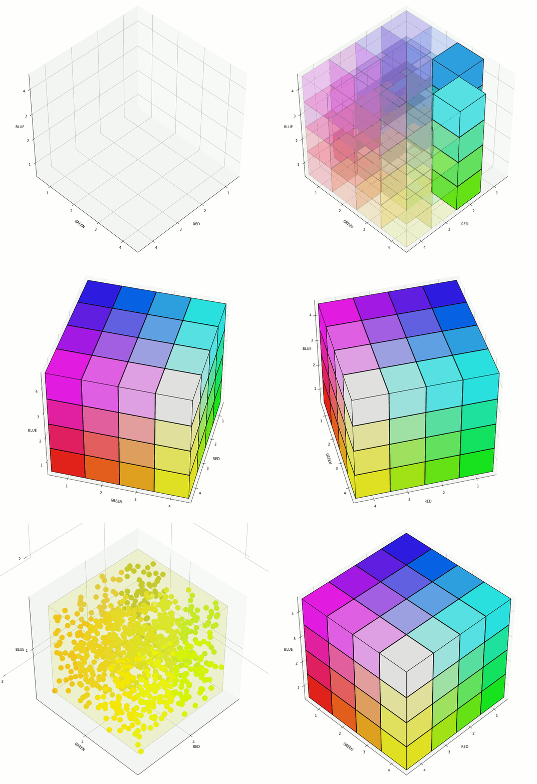
In support of some work related to color theory and linguistic relativity, I wrote some Python code to create visualizations of the RGB color space. A demo of some of the possible visualizations can be seen below (note, the animated GIF was created using GIMP):

The relevant code follows (Python 3.7):

%matplotlib inline

import matplotlib.pyplot as plt
from mpl_toolkits.mplot3d import Axes3D
from mpl_toolkits.mplot3d.art3d import Poly3DCollection
import random
import copy

def get_color_verts(r_rng, g_rng, b_rng):
    """
    Given a range in the RGB space, compiles list of vertices to be drawn.
    Used to draw the cubes representing each of the 64 defined colors.
    """
    r_min, r_max = r_rng
    g_min, g_max = g_rng
    b_min, b_max = b_rng
    # In order: r+g wrt-b, r+b wrt-g, g+b wrt-r 
    verts = [[(r_max,g_min,b_min),(r_max,g_max,b_min),(r_min,g_max,b_min),(r_min,g_min,b_min)],
             [(r_max,g_min,b_max),(r_max,g_max,b_max),(r_min,g_max,b_max),(r_min,g_min,b_max)],
             [(r_max,g_min,b_min),(r_max,g_min,b_max),(r_min,g_min,b_max),(r_min,g_min,b_min)],
             [(r_max,g_max,b_min),(r_max,g_max,b_max),(r_min,g_max,b_max),(r_min,g_max,b_min)],
             [(r_min,g_min,b_max),(r_min,g_max,b_max),(r_min,g_max,b_min),(r_min,g_min,b_min)],
             [(r_max,g_min,b_max),(r_max,g_max,b_max),(r_max,g_max,b_min),(r_max,g_min,b_min)]
            ]
    return verts

def get_color_middle(r_rng, g_rng, b_rng):
    """
    Given a range in the RGB space, returns the color represented by the center point of the cube.
    Used to draw the color of a given cube.
    """
    r_min, r_max = r_rng
    g_min, g_max = g_rng
    b_min, b_max = b_rng
    return (((r_min+r_max)/2)/255.0, ((g_min+g_max)/2)/255.0, ((b_min+b_max)/2)/255.0)

def get_random(min_val, max_val):
    return random.randint(min_val, max_val)

def get_random_color(r_rng, g_rng, b_rng):
    """
    Given a range in the RGB space, selects a random point within the cube and returns the associated color.
    Used to draw random points within each shown cube.
    """
    val = [get_random(r_rng[0], r_rng[1]),
           get_random(g_rng[0], g_rng[1]),
           get_random(b_rng[0], b_rng[1])]
    return val

def adjust_points_per_cube(orig, color_list):
    """
    Depending on the number of colors which will be drawn, adjust the number of points shown in each.
    Used to balance performance.
    """
    ret = orig
    if orig == 0:
        if not color_list or len(color_list) > 8:
            ret = 50
        elif len(color_list) == 1:
            ret = 1000
        elif len(color_list) <= 3:
            ret = 500
        elif len(color_list) <= 8:
            ret = 300    
    return ret

def get_filtered_color_list(all_colors, inc_colors):
    ret = []
    if not inc_colors:
        ret = copy.deepcopy(all_colors)
    else:
        for c in all_colors:
            if c["key"] in inc_colors:
                ret.append(c)
    return ret  
       
def set_axis_limits(ax, show_full_grid, color_list):
    """
    Calculates the limits of each axis, depending on which subset of the RGB space is being shown.
    """
    if show_full_grid:
        ax.set(xlim3d = (0, 255), ylim3d = (0, 255), zlim3d = (0, 255))
    else:
        # Get min/max for chart limits (start w/inverse)
        r_min, r_max, g_min, g_max, b_min, b_max = [255, 0, 255, 0, 255, 0]
        for c in color_list:
            r_min = min(r_min, c["r"][0])
            g_min = min(g_min, c["g"][0])
            b_min = min(b_min, c["b"][0])
            r_max = max(r_max, c["r"][1])
            g_max = max(g_max, c["g"][1])
            b_max = max(b_max, c["b"][1])
            # ax.set(xlim3d = (r_min, r_max), ylim3d = (g_min, g_max), zlim3d = (b_min, b_max))
            ax.set(xlim3d = (r_min-5, r_max+5), ylim3d = (g_min-5, g_max+5), zlim3d = (b_min-5, b_max+5))    

def draw_random_points(points_per_cube, color_list):
    for col in color_list:
        for i in range(points_per_cube):
            ci = get_random_color(col["r"], col["g"], col["b"])
            area = (15)**2
            ax.scatter(ci[0], ci[1], ci[2], 
                       color = [ci[0]/255.0, ci[1]/255.0, ci[2]/255.0], 
                       s = area)

def draw_cubes(ax, color_list, hilite_list, cube_alpha, hilite_alpha, edge_color):
    for c in color_list:
        p = Poly3DCollection(get_color_verts(c["r"], c["g"], c["b"]), alpha = cube_alpha)
        p.set_color(get_color_middle(c["r"], c["g"], c["b"]))
        if c["key"] in hilite_list:
            p.set_alpha(hilite_alpha)
        if edge_color:
            p.set_edgecolor(edge_color)
        ax.add_collection3d(p)            
            
def set_axis_tickmarks(ax, x, y, z):
    ax.set_xticks(x)
    ax.set_yticks(y)
    ax.set_zticks(z)
    
def set_axis_ticklabels(ax, x, y, z):
    ax.set_xticklabels(x)
    ax.set_yticklabels(y)
    ax.set_zticklabels(z)    

def create_color_list():
    """
    Creates a list of 64 "colors", by evenly dividing RGB space into 64 equal-sized cubes.
    This is accomplished by dividing each axis (R, G, B) into quarters.
    """
    # NOTE: A 3-character "key" is used to identify each of the 64 cubes. Used in filtering the display.
    keys_ = [["B", "G", "L", "M"],["A", "E", "I", "O"],["R", "S", "T", "V"]]
    rng_ = [[0, 63], [64, 127], [128, 191], [192, 255]]

    colors = []
    for idx_r, rng_r in enumerate(rng_):
        for idx_g, rng_g in enumerate(rng_):
            for idx_b, rng_b in enumerate(rng_):
                color = {}
                color["key"] = "{}{}{}".format(keys_[0][idx_r], keys_[1][idx_g], keys_[2][idx_b])
                color["r"] = rng_r
                color["g"] = rng_g
                color["b"] = rng_b
                colors.append(color)
    
    return colors    
 
colors = create_color_list()

show_boxes = True       # Determines whether surfaces of each defined color cube is drawn.
show_points = True     # Set to True to draw random points of example shades in each selected cube.
points_per_cube = 0     # Number of random shades to draw. Set to 0 to use defaults, which balances for performance.
box_alpha = .1         # Alpha value for all shown colors.
hilite_alpha = 1.0      # Alpha value used for colors found in hilite_cubes list.
edge_color = [0, 0, 0]  # Color used to draw the edges of vertices.
show_full_grid = False   # Setting to False will focus space on just the shown cubes.
color_filter = []       # Keys of colors to be included. Set to empty [] to include all colors.
hilite_cubes = []       # Keys of colors to hilight (will use hilite_alpha value). Ignored if empty [].

points_per_cube = adjust_points_per_cube(points_per_cube, color_filter)

x_colors = []
x_colors = get_filtered_color_list(colors, color_filter)        
            
fig = plt.figure(figsize = [14, 14])
ax = fig.gca(projection = '3d')

set_axis_limits(ax, show_full_grid, x_colors)
ax.set(xlabel = "RED", ylabel = "GREEN", zlabel = "BLUE")

ticks_ = [32, 96, 160, 223]
set_axis_tickmarks(ax, x=ticks_, y=ticks_, z=ticks_)

ticklbl_ = ["1", "2", "3", "4"]
set_axis_ticklabels(ax, x=ticklbl_, y=ticklbl_, z=ticklbl_)
         
if show_points:
    draw_random_points(points_per_cube, x_colors)
    
if show_boxes:
    draw_cubes(ax, x_colors, hilite_cubes, box_alpha, hilite_alpha, edge_color)
    
ax.view_init(45, 45)  

# fig.savefig("demo-1.png", bbox_inches = "tight")  

Lorem ipsum

I’ve recently been spending some time better understanding color theory, specifically as it relates to linguistic determinism and relativity. As I feel myself beginning to move away from this area of study, I wanted to document a few notes and observations, in case I wanted to return in the future.

The above video covers mostly notes/observations relevant to color theory and linguistic relativity. I also wanted to document some speculation and theories related to linguistic relativity, which I’ve done in the following video:

The following project pitch was submitted to the National Science Foundation ‘s (NSF) Seed Fund program on 25-Sep-2019, under the “SBIR: Artificial Intelligence (AI)” Topic Area. The project was subsequently accepted by the relevant NSF Program Director on 19-Oct-2019, resulting in an invitation to submit a full proposal for the NSF SBIR/STTR Phase I program. This invitation is valid for a period of one year, expiring on 19-Oct-2020.

Question #1

Briefly Describe the Technology Innovation.
Up to 500 words describing the technical innovation that would be the focus of a Phase 1 project, including a brief discussion of the origins of the innovation as well as an explanation as to why it meets the program’s mandate to focus on supporting research and development (R&D) of unproven, high-impact innovations.

Significant resources are expended to digitize the physical collections of Cultural Heritage Organizations, and in making these collections widely accessible and useful. The creation of associated metadata is crucial for the usability of each collection, and accounts for a significant portion of total project cost. The creation of metadata accounts for 29% of total digitization costs, with the manual nature of descriptive metadata generation being a major factor.

Despite these expenditures, the metadata found on existing collections is often incomplete, inconsistent and incorrect. Personally, this became obvious while attempting to advance a research project by leveraging some of these collections, only to be frustrated by sparse and non-standard metadata. Following this experience, I resolved to better understand and attempt to address the underlying problems.

This project aims at significantly reducing the digitization costs of cultural heritage collections, while simultaneously improving their usefulness. I believe this is attainable via the novel application of soft computing techniques, toward the following objectives:

  1. The automated generation of descriptive metadata aligned with widely used taxonomies.
  2. The temporal and spatial labeling of unidentified documents.
  3. The automated detection of errors in existing descriptive metadata.

At its core, the solution involves training a collection of classification models to recognize specific attributes of documents, covering both subject matter (e.g., “portrait”) and format (e.g., “daguerreotype”). Each classification model would be treated as a “membership function” defining the fuzzy set of documents containing that attribute.

For metadata generation, we associate each membership function with the relevant node of a standard taxonomy, for example, the Library of Congress Subject Headings (LCSH). A given document would then receive the taxonomical tags associated with each set to which it belongs. As an example, any document found to be a member of the “daguerreotype” set, would receive the LCSH tag “sh85035408”, which covers daguerreotypes.

A subset of our membership functions will define “temporally differentiable” attributes. That is to say that a document’s membership in these sets tells us something about when the document was created. With these membership functions, and a large pre-labeled dataset, we can construct temporal histograms reflecting the historical distribution of each attribute. A similar approach can be taken to understand spatio-temporal distributions, as appropriate.

These distributions can be used both to make predictions of unidentified documents (as documents will likely abide by the observed distributions), and to uncover potentially incorrect metadata via outlier identification. The specificity of our predictions can be increased by combining the distributions of multiple attributes, and by “breaking” attributes into more-specific categories.

Though some relevant research has been conducted into the application of similar techniques to subsets of this problem (e.g., the temporal identification of color photographs) it appears that little effort has been applied to the practical, systematic application of these techniques to meet the specific requirements of this domain. Given this, and the potential value of a practical solution, this is believed to be a worthy area of investment.

Question #2

Briefly Describe the Technical Objectives and Challenges.
Up to 500 words describing the R&D or technical work to be done in a Phase I project, including a discussion of how and why the proposed work will help prove that the product or service is technically feasible and/or significantly reduces technical risk. Discuss how, ultimately, this work could contribute to making the new product, service, or process commercially viable and impactful. This section should also convey that the proposed work meets definition of R&D, rather than straightforward engineering or incremental product development tasks.

It is believed that a successful phase 1 implementation can be limited in scope to processing photographs in batch, but should demonstrate an ability to:

  1. Automatically generate taxonomical tags for a representative set of descriptive metadata attributes.
  2. Make reasonable, evidence-based temporal predictions of items.
  3. Identify items which may have incorrect temporal metadata labels.

By proving these capabilities, we can demonstrate an approach to reducing the costs associated with manually creating new metadata, as well as an approach to improve the quality of existing metadata. With this promise, it is believed that we can encourage the participation of a number of target customers, whose engagement will be vital in helping guide a solution toward product-market fit.

The work involved in demonstrating these capabilities can coarsely be categorized as follows:

  1. Acquire a relatively large labeled dataset of historic photographs.
  2. Select a representative set of metadata attributes.
  3. Train membership functions for each of the selected attributes.
  4. Develop a process for automatically generating a list of taxonomical metadata labels based on set membership.
  5. Develop a process for automatically predicting temporal labels based on set membership.
  6. Develop a process for discovering erroneous labels by identifying temporal outliers.

It is generally understood that progress in soft computing is constrained by the availability of labeled data. Though some relevant research appears to have been affected by this constraint, it is not believed to be a significant impediment to our progress. This is due to the efforts of a handful of organizations focused on the aggregation and standardization of the metadata associated with many relevant digital collections, for example, the Digital Public Library of America (DPLA). Their work largely eliminates the risk that would otherwise be inherent in #1 (above).

Therefore, based on current understanding, it is believed that most of our technical risk lies in items #3, #5, and #6.

Regarding the training of membership functions, it is unknown to what extent this will require the use of fine-grained classification techniques. Given the relative immaturity of proven fine-grained techniques (as compared to coarse-grained approaches) this may require additional work to assess and implement an effective solution.

Regarding the prediction of temporal labels, there exists limited relevant research and no known practical implementations. Though we believe the use of observed distributions, in combination with approaches outlined by prior research efforts, will result in a viable solution, a rigorous empirical assessment of the approach is warranted. Given the availability an existing labeled dataset, such an assessment appears feasible.

Technically, the automatic identification of erroneous labels is closely tied to the work of predicting temporal labels, and shares much of the same technical risk. The quantitative assessment of the approach, though, appears less obvious, and may require coordination with the publishing organizations for confirmation.

Given the study required, and the novel application of emerging techniques within this domain, the described work appears well aligned with the NSF’s stated R&D requirements.

Question #3

Briefly Describe the Market Opportunity.
Up to 250 words describing the customer profile and pain point(s) that will be the near-term commercial focus related to this technical project.

The initial customer focus includes organizations involved in the digitization or aggregation of cultural heritage collections:

  • Cultural Heritage Organizations (CHOs), including libraries, museums, archives, and historical societies.
  • Aggregation Organizations, e.g., the Digital Public Library of America (DPLA).
  • Digitization Service Organizations, e.g., Everpresent, and Backstage Library Works.

Digitization projects include significant manual effort related to the curation of descriptive metadata. Requirements for this curation process are typically defined by the publishing organization, though work can fall to any of the listed organization types, depending on the structure of the project.

The inherent manual effort of this process leads to higher costs and potential errors. Given the constrained budgets of these projects, this represents the significant pain point we hope to address.

In estimating the number of CHOs in the US, we determine there to be roughly:

  • 9,000 public libraries.
  • 3,000 academic libraries.
  • 5,000 historical societies and preservation offices.

Though a full picture of digitization project expenditures is unclear, grants awarded by the National Endowment for the Humanities (NEH) and the Council on Library and Information Resources (CLIR) is instructive:

  • NEH awarded $230,000,000 from 2008-2017, initiated by their related divisions (the offices of Preservation and Access, and Digital Humanities).
  • CLIR has awarded $4,000,000 annually since 2015, as part of their Digitizing Hidden Collections program.

Though not part of our initial focus, we believe that opportunity may also exist with international CHOs, collection management software (CMS) providers, and non-CHO archives.

This post documents the code used to compare model iterations, as described in the post “Bootstrapping Model Data“. The code is written in Python 3.7.

Input

This code is currently comparing the results of 2 models. The results for each model are stored in a JSON file, which contains the model’s prediction for each image in my full image set.

An example of this JSON file follows:

[
    {
        'path': 'D:\\Roots\\oai-images\\00000000-0000-0000-0000-000000000000-roots-1.jpeg',
        'value': 'negative',
        'conf': 0.72014
    },
    ....
]

This snippet shows the stored prediction for one image. Each saved prediction includes:

  • The path of the image used to make this prediction.
  • The value of the prediction made by the model. In this example, value will either be “positive” or “negative” depending on whether the image contains a picture of a bridge or not (respectively).
  • The confidence of the model’s prediction (conf).

Output

For each model, I’m outputting some very basic stats of the predictions (output_stats) and a histogram which shows the spread of the predictions (plot_histogram):

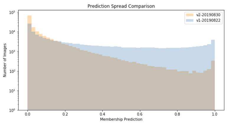
Next, I’m outputting a combined histogram of all models (plot_histogram):

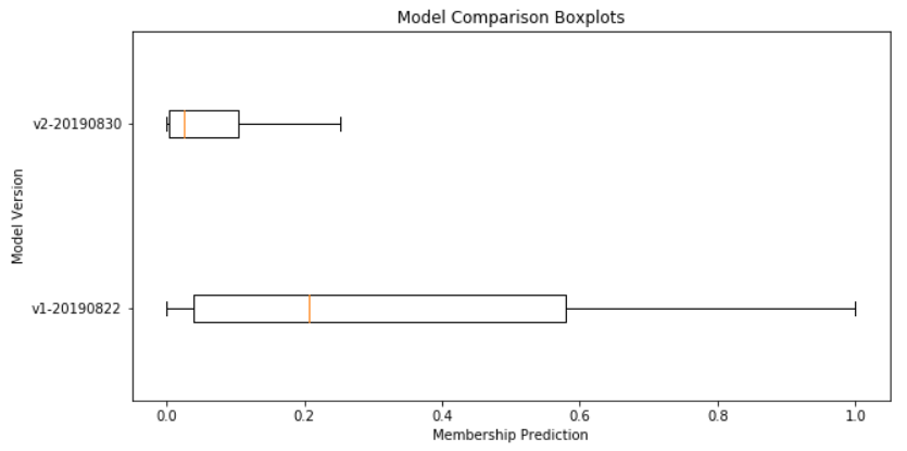
Finally, I’m also plotting the results of all models as a box plot (plot_boxplot):

Code

Here is the code used to generate these visualizations, in Python 3.7. Note that this is prototype, and not production-ready…

import matplotlib.pyplot as plt
import json

def get_json_from_path(file_path):
    json_data = json.loads(open(file_path).read())
    return json_data


def get_membership_value(item):
    if item["value"] == "negative":
        return 1 - item["conf"]
    else:
        return item["conf"]


def plot_histogram(data, title, xlabel, ylabel, label, color, log = False):
    plt.figure(figsize = (10, 5))
    _ = plt.hist(data, bins = 50, log = log, histtype = "stepfilled", alpha = 0.3, label = label, color = color)

    plt.legend(prop={'size': 10})
    plt.ylim(bottom=1)
    plt.title(title)
    plt.xlabel(xlabel)
    plt.ylabel(ylabel)
    plt.show()   

    
def plot_boxplot(data, title, xlabel, ylabel, label):
    plt.figure(figsize = (10, 5))
    _ = plt.boxplot(data, labels = label, vert = False, showfliers = False)
    plt.title(title)
    plt.xlabel(xlabel)
    plt.ylabel(ylabel)
    plt.show()


def output_stats(data, name):    
    total_count = len(data)
    pos_count = 0
    pos_gt90_count = 0
    for item in data:
        if item > 0.5:
            pos_count += 1
            if item >= 0.9:
                pos_gt90_count += 1
    
    print("Stats for {}:".format(name))
    print("  Total Items: {}".format(total_count))
    print("  Positive Items: {0} ({1:.2f}%)".format(pos_count, pos_count / total_count * 100))
    print("  Above 90%: {0} ({1:.2f}%)".format(pos_gt90_count, pos_gt90_count / total_count * 100))

 
v1res_path = r"D:\Roots\model-predictions\roots-Contains-Structure-Bridge-20190822-vl0p23661.json"
v2res_path = r"D:\Roots\model-predictions\roots-Contains-Structure-Bridge-20190830-vl0p29003.json"

v1_results = list(map(get_membership_value, get_json_from_path(v1res_path)))
v2_results = list(map(get_membership_value, get_json_from_path(v2res_path)))

data = (v1_results, v2_results)
names = ("v1-20190822", "v2-20190830")
colors = ("steelblue", "darkorange")

for i in range(0, len(names)):
    output_stats(data[i], names[i])
    plot_histogram(data[i], "{} Prediction Spread".format(names[i]), "Membership Prediction", "Number of Images", label = names[i], log = True, color = colors[i])

plot_histogram(data, "Prediction Spread Comparison", "Membership Prediction", "Number of Images", label = names, log = True, color = colors)

plot_boxplot(data, "Model Comparison Boxplots", "Membership Prediction", "Model Version", label = names)

As part of an active project, I’m exploring ways to iteratively build a dataset of images for use in training classification models.

This article documents some early activity, but does not reach conclusion on any repeatable processes.

Problem Overview

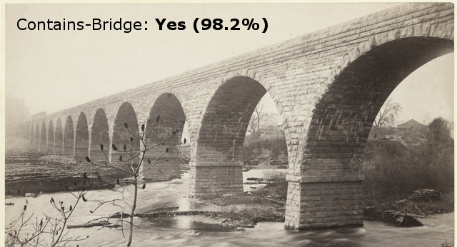
For this example I’m working to build an image classification model which is able to identify whether a picture contains a bridge:

This will be one of a larger set of models, trained to act as membership functions to identify various types of structures. For example, water towers, lighthouses, etc.

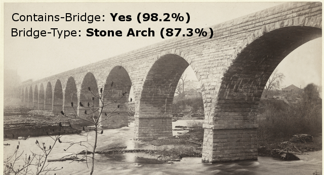
Eventually, once we have a large-enough dataset, another model will be trained to more-specifically classify the type of bridge shown in the image (e.g., truss, suspension, etc.):

Given the large number of images required to train an effective model of this type, I need to find a more-efficient process for identifying and labeling images to include in a training dataset.

Source of Data

The context for my larger project is identifying historical photographs. Given this, most of my training data will be coming from the collections of historical societies, universities, and other similar organizations.

Though I’ll save the details for a future post, there are a couple of standards used to provide programmatic access to these digital collections. The one I’ve focused on is called the “Open Archives Initiative Protocol for Metadata Harvesting” (OAI-PMH).

I am maintaining a list of organizations providing OAI-PMH access to their collections, and am downloading images via this standard. At the time of this writing, I’ve downloaded ~150k images for use in model training and am continuing to grow this set.

Iteration #1

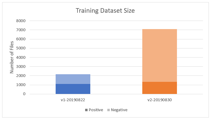
For the first training iteration, I manually labeled a set of 2,172 images. Half of these images contained bridges, and the other half did not.

I then did a random 80/10/10 split of this data for Validation/Training/Test. This resulted in 1,736 images for training, 216 images for validation, and 220 for testing.

A pre-trained MobileNetV2 model was then trained (via transfer learning) over 75 epochs, to reach an accuracy of ~89% against the Test dataset. For the rest of this article, this version of the model will be named v1-20190822.

The plan was then to use this model to more-efficiently build a larger training dataset. The larger dataset would be pulled from the images I had downloaded from historical societies…

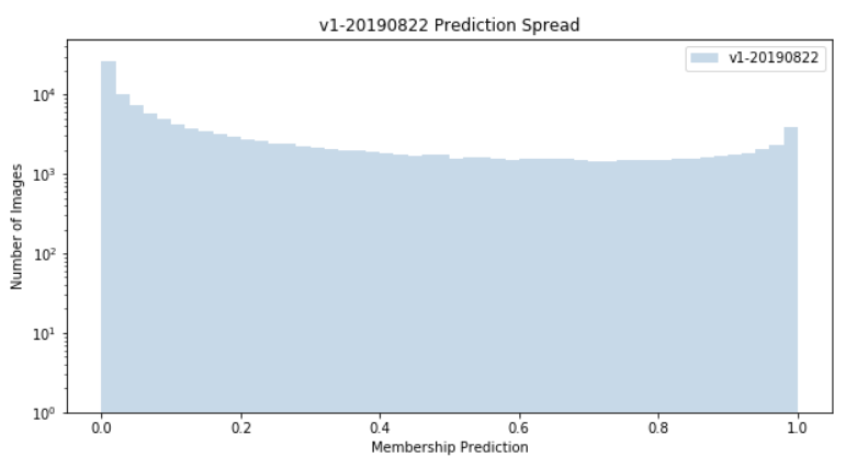
At this point, I had 145,687 total candidate images downloaded. I ran the model against all images and found:

  • 42,733 images (29.33%) were labeled as containing a bridge.
  • 11,880 images (8.15%) were labeled as +90% confident in containing a bridge.

A histogram of all predictions is shown below. Note that, in this visualization, a value of “0” represents 100% confidence that the image does not contain a bridge:

In reality, this first model performed very poorly. Many images were being incorrectly classified, and in non-intuitive ways — for example, many portraits were being classified as containing bridges…

In hindsight, this first iteration could have been better if I’d done a better job at compiling the negative images (i.e., those not containing a bridge). Nearly all of these images were external, architectural shots, which led to model confusion when it encountered a more normal distribution of photograph types.

This would be resolved in future iterations.

Iteration #2

To build the training set for the second version of the model, I ran the first model against all 145,000 candidate images, and found those images labeled as containing bridges with at least 92% confidence.

This left me with 7,107 images. After manually labeling these images, I was left with 1,346 photos containing bridges (“positive”), and 5,761 which did not (“negative”). A comparison of the size of datasets, between iteration #1 and #2, follows:

I used this new dataset to train a new version of the model, following the same process and architecture as previously. After 75 epochs, the model reached ~88% accuracy against the Test portion of the dataset.

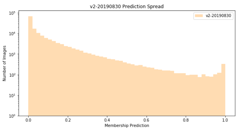
I then ran this second version of the model (named v2_20190830) against the full set of 145,687 candidate images and found:

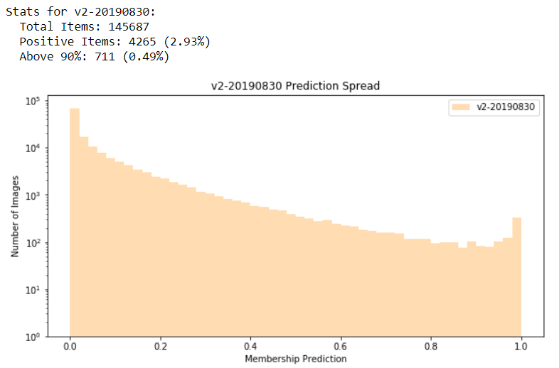
  • 4,265 images (2.93%) were labeled as containing a bridge.
  • 711 images (0.49%) were labeled as +90% confident in containing a bridge.

A histogram of all predictions from this second model is shown below:

Qualitatively, this model performed much better than the first, and most of the incorrect classifications were very intuitive — for example, many false-positives were non-bridge structures that contained elements that looked like trusses or arches, which are very common in bridge designs.

Model Comparison

As I iterate this process, and train against larger datasets, I would expect my models to become much more discriminating. In the early iterations, this likely means that a smaller percentage of total images are included in the “positive” class.

Overlaying the histograms of these first two models is interesting, as it shows evolution in that direction:

Another way to view this information would be to plot the same information in box plots (here, I’ve removed the outliers for visual clarity):

Next Steps

I’m actively working on the third iteration of the training dataset, and will update in a future post.

Toward this end, I’m downloading more candidate images from historical societies, and will be running the v2 model against this larger candidate set to grow my dataset, ahead of training the next model.

More to come!